Does negative wealth shock cause an increase in all-cause mortality?

The profile picture credits to the artist @feliciachiao.

Note: The codes are too long to display in this blog so, I have inlcuded all the codes here

A sudden negative wealth shock may cause significant increase of health risk. In this post, I will use causal inference methods to analyze the question, does negative wealth shock cause an increase in all-cause mortality?

1. Data preparation

I will use the Health and Retirement Study (HRS) data. HRS data is a nationally representative prospective longitudinal cohort study of US adults aged 51 or higher. I used the original HRS cohort, born in 1931 through 1941. I collected the data until 2016. At each interview, participants were provided a written informed consent document and asked to consent orally. For consistency, I only included cases that have first interview in 1992.

I have cleaned and aggregated HRS multi-wave longitudinal data, identified negative wealth shock, and integrated mortality data. The data size is too large to be uploaded to github, so if you want to check out the cleaned data, please let me know. If you want to see how I clean the data from sketch, you can take a look at my github. I have to say, 80% percent the time I spent in this project was data cleaning 😢😭. Thankfully, the tidyverse package make the data cleaning work less painful.

Later, based on this paper, I selected out 11 baseline covariates including age at enrollment, self-reported sex, self-reported race, whether is Hispanic or not, educational attainment, health behaviors including smoking status, alcohol consumption, physical activity and body mass index. I also included 2 indicators: (1) financial risk aversion and (2) expectation of leaving a bequest upon death. Here is the code book for the baseline covariates:

• Age at 1992 interview: AAGE from tracker file (continuous)
• self-reported sex: RAGENDER from hrs file (categorical)
• self-reported race/ethnicity: RARACEM from hrs file (categorical)
• Whether Hispanic: RAHISPAN from hrs file (categorical)
• educational attainment: RAEDYRS from hrs file (continuous)
• smoking status: R1SMOKEN from hrs (categorical)
• alcohol consumption: R1DRINKR from hrs (categorical)
• physical activity: R1VIGACT from hrs (categorical)
• BMI: R1BMI from hrs (continuous)
• Financial risk aversion: R1RISK from hrs (categorical)
• leave a bequest: R1BEQLRG from hrs (categorical)

I generated the box plot of the three continuous covaiates between people experienced negative wealth shock and people didn’t experience negative wealth shock.

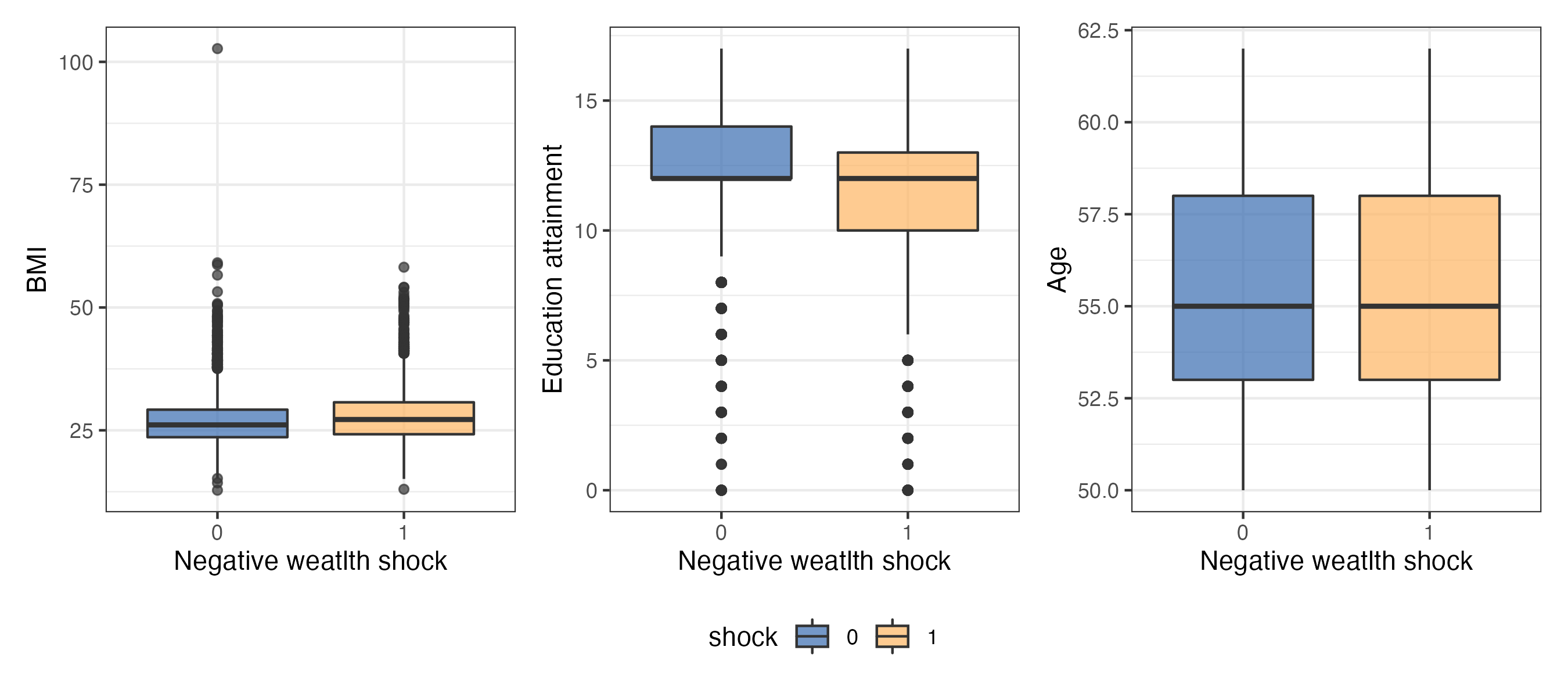
From the box plot above, we can see that age and bmi are pretty balancing among different group. However, people that didn’t experience any negative wealth shock tends to have higher education level or longer education attainment. Thus, matching is an important step to measure the causal effect between negative wealth shock and all-cause mortality

2. Matching with baseline covariates

After removing missing values, we have 8409 cases remaining. In the 8409 cases, 3162 cases experienced at least one negative wealth shock (treatment group) while 5247 never experienced any negative wealth shock (control group). I used the 11 covariates to calculate propensity score and to the matching.

2.1 Propensity Score Caliper Matching

If you are not familiar with what is matching, here is a great review.

\(\theta\)

The R package, optmatch, is a very powerful tool to implement pair-matching and full-matching based on user-specified distance metric. We want to match the 3162 cases in treatment group to the cases in the control group. We used pair matching. The R package, optmatch, took a very long time, like forever, to finish matching the 3162 cases in the treatment group to the 5247 cases in the control group. So, we divided the data into two piece, and did matching in each subset data. You can check my R codes here.

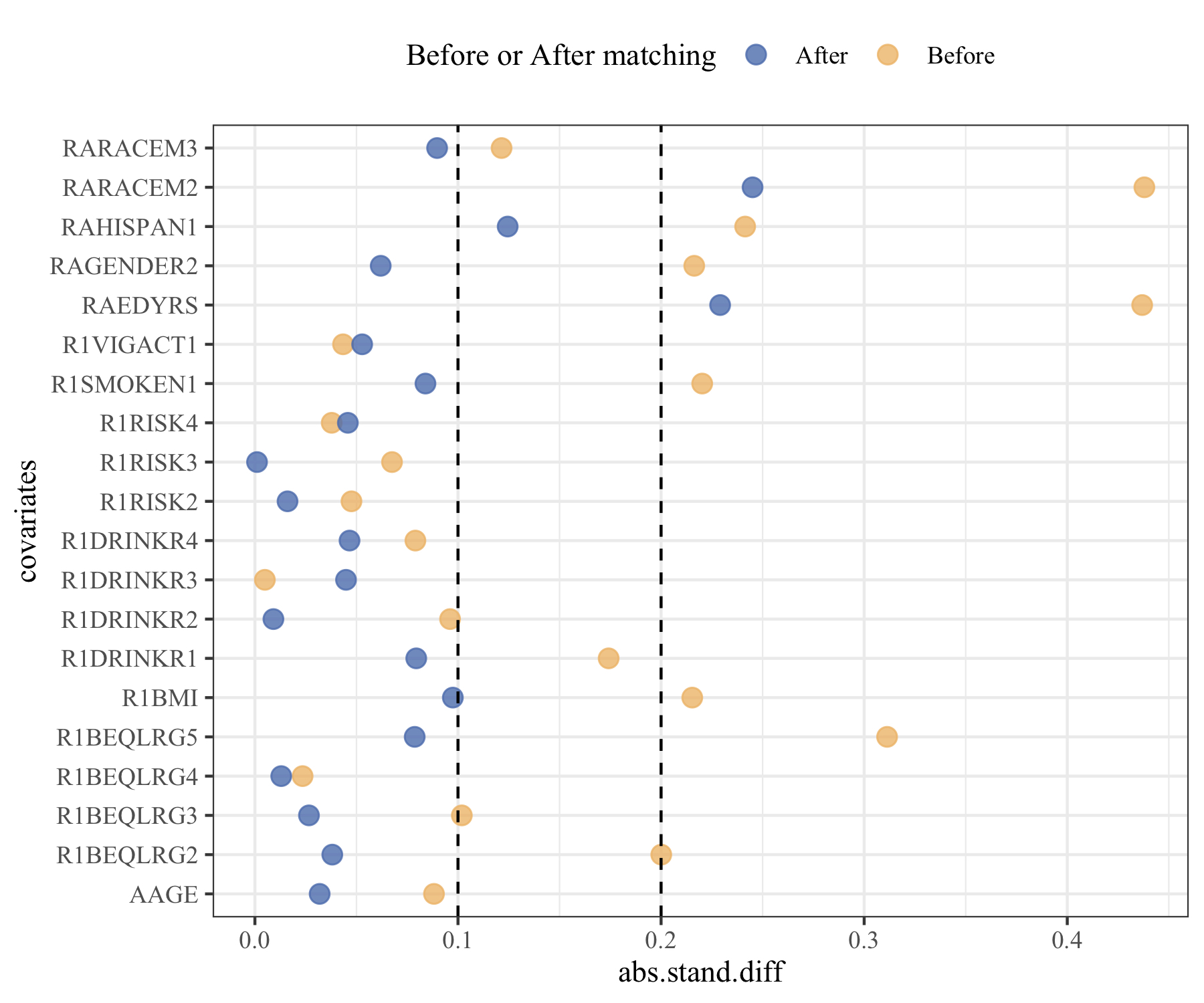
2.2 Matching Performance

Next we want to see how’s the performance of the matching. We can examine the standardized differences. The following figure shows the standardized differences for each covariate before and after matching. The standardized differences for most covariates reduce significantly after matching.

2.3 Estimated risk difference in matched set

Finally, the risk difference between treatment group and control group can be estimated by using a two sample paired t-test. The estimated risk difference is 0.0404. The 95% CI is [0.018, 0.063]. This is a very interesting result. So the negative wealth shock cause an increase in all-cause mortality. However, we need to know this result is based on the assumption that we have observed all the confounders. To measure the effect of unobserved confounders, we may need to conduct sensitivity analyses.